
Autoregressive Conditional Heteroscedasticity (ARCH) Models
ARCH models, introduced by Engle (1982), are a class of statistical models for time series data that explicitly model the time-varying volatility (conditional heteroscedasticity) of the error term. They are particularly useful for analyzing financial time series, where volatility clustering is a common feature.
Basic Idea
The fundamental idea behind ARCH models is that the variance of the error term in a regression model depends on the past values of the squared error terms. In other words, large squared errors in the past imply a higher variance today, reflecting the phenomenon of volatility clustering.
ARCH(q) Model
The ARCH(q) model specifies that the conditional variance of the error term at time t depends on the q most recent squared error terms. The model is defined as follows:
- Mean Equation:
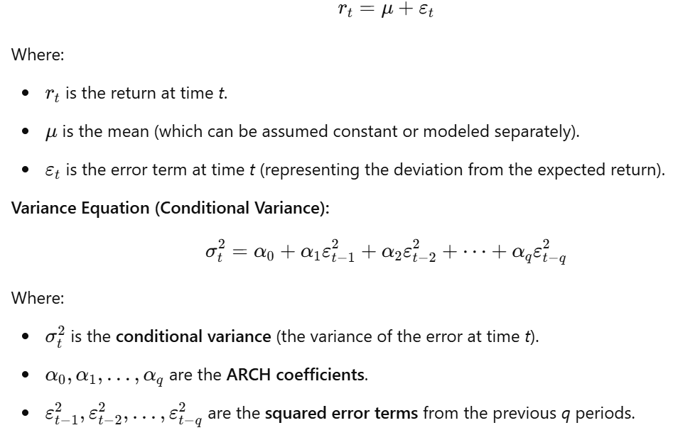
-
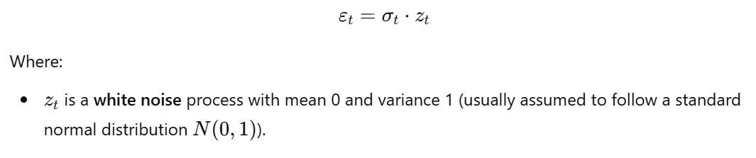
Error Term Distribution:

Key Assumptions and Properties
-
Non-Negativity Constraints: The coefficients
α_0, α_1, ..., α_qmust be non-negative to ensure that the conditional variance is always positive (σ_t^2 > 0). - Stationarity Condition: For the ARCH(q) process to be stationary, the coefficients must also satisfy certain conditions that ensure the variance does not explode over time.
-
Unconditional Variance: The unconditional variance of
ε_tis constant but higher than the conditional variance at times of low volatility. -
Volatility Clustering: ARCH models capture volatility clustering because large shocks (large
ε_{t-i}^2) in the past lead to a higher conditional variance today, implying higher volatility. - Symmetric Response: ARCH models respond symmetrically to positive and negative shocks. A large positive shock and a large negative shock of the same magnitude will have the same impact on the conditional variance. This is a limitation, as it does not capture the leverage effect.
Example: ARCH(1) Model
The ARCH(1) model is the simplest ARCH model, where the conditional variance depends only on the most recent squared error term:
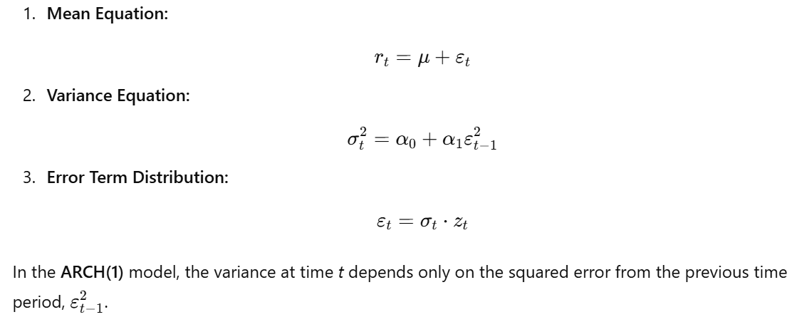
The ARCH(1) model is stationary if 0 < α_1 < 1.
Estimation of ARCH Models
The parameters of ARCH models (μ, α_0, α_1, ..., α_q) are typically estimated using maximum likelihood estimation (MLE). This involves finding the parameter values that maximize the likelihood of observing the given data, given the ARCH model specification.
Model Selection
The order q of the ARCH model can be selected using information criteria, such as the AIC or BIC, or by examining the partial autocorrelation function (PACF) of the squared residuals from a simpler model (e.g., an ARMA model for the mean).
Limitations of ARCH Models
- Symmetric Response: ARCH models do not capture the asymmetric response of volatility to positive and negative shocks (the leverage effect).
- Parameter Restrictions: The non-negativity constraints on the coefficients can be restrictive.
- High Order Required: In practice, ARCH models often require a high order (q) to adequately capture the persistence of volatility. This can lead to a large number of parameters to estimate.
Extensions of ARCH Models
Several extensions of ARCH models have been developed to address these limitations, including:
- GARCH (Generalized ARCH) Models: Allow the conditional variance to depend on both past squared error terms and past conditional variances.
- EGARCH (Exponential GARCH) Models: Capture the asymmetric response of volatility to positive and negative shocks.
- TARCH (Threshold ARCH) Models: Also capture asymmetric effects.
- FIGARCH (Fractionally Integrated GARCH) Models: Capture long memory in volatility.
Conclusion
ARCH models provide a framework for understanding and modeling time-varying volatility in financial time series. While they have some limitations, they are a significant improvement over traditional volatility measures that assume constant volatility. ARCH models are widely used in risk management, option pricing, and other financial applications.