
Introduction to Univariate Time Series
A time series is a sequence of data points, measured typically at successive points in time or over successive periods. Examples include daily stock prices, monthly inflation rates, and annual GDP growth. A univariate time series involves only one variable observed over time. Analyzing these series involves understanding their patterns, dependencies, and statistical properties to make forecasts or draw inferences about the underlying process generating the data.
Key Concepts in Univariate Time Series Analysis
-
Stationarity: A fundamental concept in time series analysis. A time series is said to be strictly stationary if its statistical properties are unaffected by shifts in time. In other words, the joint distribution of any set of observations
(X_t1, X_t2, ..., X_tn)is the same as the joint distribution of(X_{t1+k}, X_{t2+k}, ..., X_{tn+k})for any integer k.- A weaker form of stationarity, often called covariance stationarity or weak stationarity, requires only that the mean and autocovariance of the series are constant over time and that the autocovariance depends only on the lag between the observations.
- Most time series models assume at least weak stationarity. Transformations like differencing can often be used to make a non-stationary series stationary.
-
Autocorrelation: Measures the linear relationship between a time series and its lagged values. The autocorrelation function (ACF) plots the autocorrelation at different lags.
-
Partial Autocorrelation: Measures the correlation between a time series and its lagged values, after removing the effects of the intermediate lags. The partial autocorrelation function (PACF) plots the partial autocorrelation at different lags.
-
White Noise: A time series is considered white noise if its values are uncorrelated and have zero mean and constant variance. White noise is unpredictable and often serves as a building block for more complex time series models.
The Lag Operator
The lag operator (denoted by L) is a mathematical operator that shifts a time series back one period. It's a convenient notation for expressing time series relationships and for manipulating time series equations.
Definition
Applying the lag operator L to a time series X_t gives:
L X_t = X_{t-1}
In other words, L shifts the series back by one period.
Properties and Uses
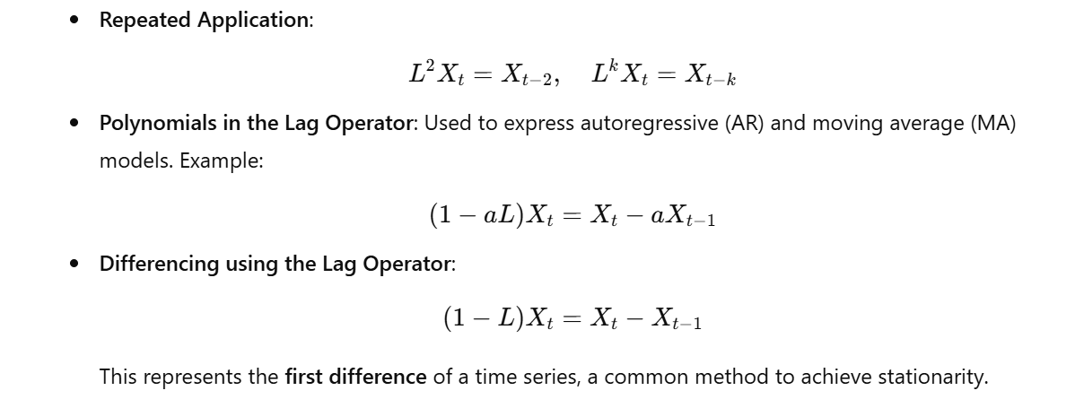
Repeated Application:Applying the lag operator multiple times shifts the series back multiple periods:
L^2 X_t = L (L X_t) = L X_{t-1} = X_{t-2}
L^k X_t = X_{t-k}
Polynomials in the Lag Operator:The lag operator can be used to express polynomials inL, which are useful for representing autoregressive (AR) and moving average (MA) models. For example:(1 - aL) X_t = X_t - a X_{t-1}Differencing:The first difference of a time series can be expressed using the lag operator:(1 - L) X_t = X_t - X_{t-1}Backshift Notation:Sometimes the lag operator is called the backshift operator, denoted byB. Therefore,B = L.
Example: AR(1) Model
An autoregressive model of order 1, AR(1), can be written as:
X_t = φ X_{t-1} + ε_t
Where:
X_tis the time series at timetφis the autoregressive coefficientε_tis a white noise error term
Using the lag operator, this can be rewritten as:
X_t = φ L X_t + ε_t
X_t - φ L X_t = ε_t
(1 - φ L) X_t = ε_t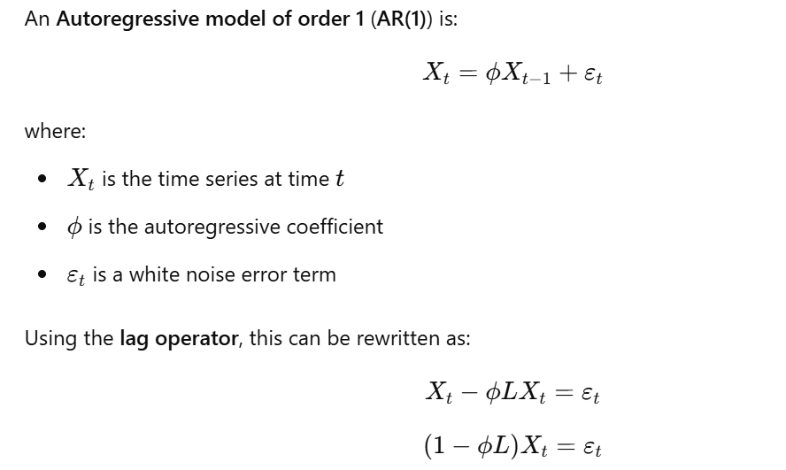
Importance
The lag operator provides a compact and powerful way to represent and manipulate time series models. It simplifies the algebra of time series and is essential for understanding AR, MA, and ARMA models.