
Labour Cost Variance
Labour Cost Variance (LCV)
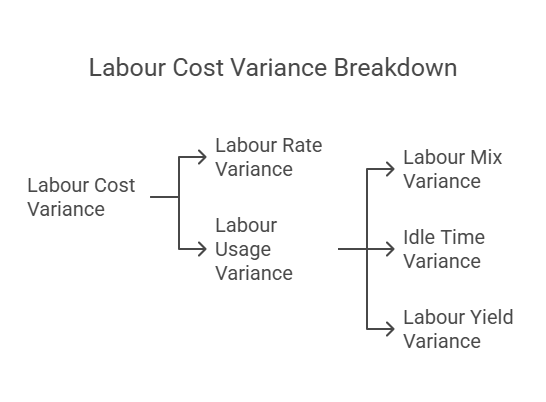
The Labour Cost Variance (LCV) measures the difference between the STANDARD COST of direct labor allowed for the ACTUAL OUTPUT achieved and the ACTUAL COST of direct labor incurred. In simpler terms, it shows how much more or less you spent on labor compared to what you expected based on your standards.
Formula
The LCV is calculated using the following formula:
- Labour Cost Variance(LCV) = Std labour cost of actual output(SC) - Actual labour cost(AC)
On further expansion:
- LCV = (Standard Hours for Actual Output * Standard Rate per Hour) - (Actual Hours * Actual Rate per Hour)
Or, more concisely:
- LCV = (SH * SR) - (AH * AR)
Where:
- SH: Standard Hours allowed for the actual output. This is the number of labor hours that should have been used to produce the actual number of units, according to your standards.
- SR: Standard Rate per hour. This is the expected hourly labor rate.
- AH: Actual Hours worked. This is the actual number of labor hours spent in production.
- AR: Actual Rate per hour. This is the actual hourly labor rate paid.
Interpretation
- Positive LCV (Favorable): A positive LCV indicates that the actual labor cost was lower than the standard labor cost. This is a favorable variance, meaning you spent less on labor than expected.
- Negative LCV (Unfavorable): A negative LCV indicates that the actual labor cost was higher than the standard labor cost. This is an unfavorable variance, meaning you spent more on labor than expected.
Example
Let's break down the provided example:
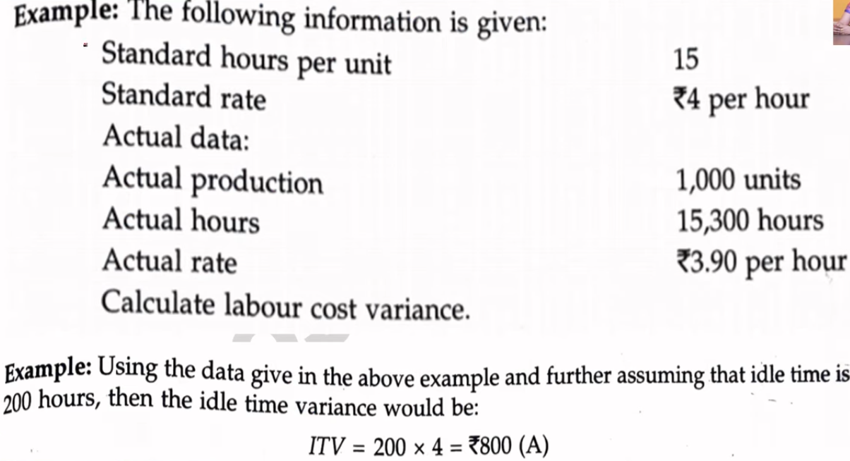
Given Data:
- Standard hours per unit = 15 hours
- Standard rate per hour = ₹4
- Actual production = 1,000 units
- Actual hours = 15,300 hours
- Actual rate per hour = ₹3.90
Calculation:
-
Standard Hours for Actual Output (SH): 1,000 units * 15 hours/unit = 15,000 hours
-
Standard Labour Cost (SC): 15,000 hours * ₹4/hour = ₹60,000
-
Actual Labour Cost (AC): 15,300 hours * ₹3.90/hour = ₹59,670
-
Labour Cost Variance (LCV): ₹60,000 - ₹59,670 = ₹330
Result and Interpretation:
The LCV is ₹330. This is a favorable variance. It means the company spent ₹330 less on labor than expected for the actual production of 1,000 units.
Further Analysis
While the LCV gives the overall variance, it's helpful to break it down further into two components:
- Labour Rate Variance: This looks at the difference between the standard rate and the actual rate.
- Labour efficiency Variance: This looks at the difference between the standard hours allowed and the actual hours worked.
Labour Rate Variance (LRV)
The Labour Rate Variance (LRV) measures the portion of the total labour cost variance that is specifically caused by the difference between the STANDARD LABOUR RATE and the ACTUAL LABOUR RATE paid. It isolates the impact of wage rate fluctuations, independent of the number of hours worked.
Formula
The LRV is calculated using the following formula:
- LRV = (Standard Rate - Actual Rate) * Actual Hours
Or, more concisely:
- LRV = (SR - AR) * AH
Where:
- SR: Standard Rate per hour. This is the expected hourly labor rate.
- AR: Actual Rate per hour. This is the actual hourly labor rate paid.
- AH: Actual Hours worked. This is the actual number of labor hours spent in production.
Interpretation
- Positive LRV (Favorable): A positive LRV indicates that the actual rate paid was lower than the standard rate. This is a favorable variance.
- Negative LRV (Unfavorable): A negative LRV indicates that the actual rate paid was higher than the standard rate. This is an unfavorable variance.
Example
Let's use the provided example:
Given Data:
- Standard rate per hour (SR) = ₹4
- Actual rate per hour (AR) = ₹3.90
- Actual hours worked (AH) = 15,300 hours
Calculation:
LRV = (₹4 - ₹3.90) * 15,300 LRV = ₹0.10 * 15,300 LRV = ₹1,530
Result and Interpretation:
The LRV is ₹1,530. This is a favorable variance. It means that the company paid ₹1,530 less for labor than expected, solely due to the lower actual hourly rate.
Reasons for Labour Rate Variance
Several factors can contribute to a labour rate variance:
-
Changes in Basic Wage Rates: Fluctuations in market wage rates, industry agreements, or changes in minimum wage laws can affect the actual labor rate.
-
Different Methods of Wage Payment: Changes in the way wages are calculated (e.g., from hourly to piece-rate or vice versa) can lead to rate variations.
-
Employing Workers of Different Grades: If workers of different skill levels or pay grades are used than those specified in the standard, it will affect the actual labor rate. For example, using a more experienced (and thus more expensive) worker for a task designed for a less experienced worker would cause an unfavorable variance.
-
Unscheduled Overtime: Unexpected overtime work, which is often paid at a premium rate, can lead to a higher actual labor rate.
-
New Workers Not Being Paid Full Rates: Trainees or new hires might be paid at lower rates than experienced workers, resulting in a favorable variance.
Labour Efficiency Variance (LEV)
The Labour Efficiency Variance (LEV), also known as the Labour Time Variance, measures the portion of the total labour cost variance that is caused by the difference between the STANDARD LABOUR HOURS allowed for the actual output and the ACTUAL LABOUR HOURS worked. It isolates the impact of using more or fewer labour hours than expected, independent of wage rate fluctuations.
Formula
The LEV is calculated using the following formula:
- LEV = (Standard Hours for Actual Output - Actual Hours) * Standard Rate
Or, more concisely
- LEV = (SH - AH) * SR
Where:
- SH: Standard Hours allowed for the actual output. This is the number of labor hours that should have been used to produce the actual number of units, according to your standards.
- AH: Actual Hours worked. This is the actual number of labor hours spent in production.
- SR: Standard Rate per hour. This is the expected hourly labor rate. It's important to use the standard rate here, as we're isolating the impact of time/efficiency differences, not rate differences.
Interpretation
- Positive LEV (Favorable): A positive LEV indicates that fewer actual hours were worked than the standard hours allowed for the actual output. This is a favorable variance.
- Negative LEV (Unfavorable): A negative LEV indicates that more actual hours were worked than the standard hours allowed for the actual output. This is an unfavorable variance.
Example
Using the provided example:
Given Data:
- Standard hours per unit = 15 hours
- Standard rate per hour = ₹4
- Actual production = 1,000 units
- Actual hours = 15,300 hours
Calculation:
-
Standard Hours for Actual Output (SH): 1,000 units * 15 hours/unit = 15,000 hours
-
Labour Efficiency Variance (LEV): (15,000 hours - 15,300 hours) * ₹4/hour LEV = (-300 hours) * ₹4/hour LEV = -₹1,200
Result and Interpretation:
The LEV is -₹1,200. This is an unfavorable variance. It means that 300 more labor hours were worked than the standard allowed for the actual output, resulting in an additional cost of ₹1,200 (at the standard rate).
Reasons for Labour Efficiency Variance
Several factors can contribute to a labour efficiency variance:
-
Poor Working Conditions: Inadequate lighting, ventilation, excessive heat or cold, and other uncomfortable or unsafe working conditions can reduce worker productivity and lead to longer work times.
-
Defective Tools and Machinery: Malfunctioning or poorly maintained equipment can cause delays, errors, and rework, requiring more labor hours.
-
Inefficient Workers: Lack of skill, experience, or motivation among workers can result in slower work pace and lower efficiency.
-
Incompetent Supervision: Poor supervision, lack of clear instructions, or inadequate support can hinder worker efficiency.
-
Use of Defective or Non-Standard Materials: If materials are of poor quality or don't meet specifications, workers may have to spend extra time working around these issues, leading to inefficiencies.
Idle Time Variance (ITV)
The Idle Time Variance (ITV) is a specific component of the Labour Efficiency Variance. It measures the cost of unproductive labor time caused by abnormal or avoidable reasons, such as machine breakdowns, power failures, strikes, material shortages, or other similar disruptions. It isolates the cost of labor hours for which employees are paid but are not actively working on production.
What is Idle Time?
Idle time refers to the period during which workers are available for work but are unable to perform their assigned tasks due to factors beyond their control. It's important to distinguish idle time from planned downtime (e.g., breaks, scheduled maintenance), which is usually included in standard labor hours. The ITV focuses specifically on unplanned and unproductive idle time.
Formula
The Idle Time Variance is calculated as:
- Idle Time Variance = Idle Hours * Standard Rate
Or, more concisely:
- ITV = IH * SR
Where:
- IH: Idle Hours. This is the number of hours during which workers were idle due to abnormal or avoidable causes.
- SR: Standard Rate per hour. This is the expected hourly labor rate. We use the standard rate because the ITV reflects the cost of unproductive labor, not necessarily the actual cost.
Interpretation
- Positive ITV (Unfavorable): A positive ITV represents an unfavorable variance. It shows the additional labor cost incurred due to idle time. The higher the idle time, the higher the cost. Note that because idle time is inherently unproductive, a "positive" variance is bad.
- Negative ITV (Favorable): While technically possible to have "negative" idle time (e.g., if some previously recorded idle time is later determined to have been productive), in practice, the ITV is almost always positive (unfavorable) or zero. A zero ITV would mean there was no unplanned idle time.
Labour Mix Variance (Gang Composition Variance)
The Labour Mix Variance, also known as the Gang Composition Variance, is similar in concept to the Material Mix Variance. It arises when a company uses different grades or types of workers (e.g., skilled, semi-skilled, unskilled) for a particular job, and the actual proportion of each grade used differs from the standard proportion specified. This variance measures the cost impact of this deviation in the labor mix.
When Does it Occur?
The Labour Mix Variance is relevant only when:
- More than one grade or type of worker is employed for the same task.
- There's a standard or predetermined mix of these worker grades specified.
- The actual mix of worker grades used deviates from this standard mix.
Formula
The Labour Mix Variance is calculated as:
- Labour Mix Variance = (Revised Standard Hours - Actual Hours) * Standard Rate
Or, more concisely:
-
LMV = (RSH - AH) * SR Where:
-
RSH: Revised Standard Hours. This is the standard number of hours that should have been worked by each grade of worker, given the actual total labor hours worked. It's not the overall standard hours for the output; it's the standard mix applied to the actual total hours.
-
AH: Actual Hours worked by each grade of worker.
-
SR: Standard Rate per hour for each grade of worker. It's critical to use the standard rate for each specific grade of worker.
Calculating Revised Standard Hours (RSH)
The RSH is calculated for each grade of worker. It represents what the standard hours for each grade would have been if the actual total labor hours were distributed according to the standard mix.
-
Calculate the total actual hours worked: Sum the actual hours worked by all grades of workers.
-
Calculate the standard proportion for each grade: Determine the percentage of total labor hours that each grade should have worked, according to the standard mix.
-
Calculate the revised standard hours for each grade: Multiply the total actual hours worked by the standard proportion for each grade.
Interpretation
- Positive LMV (Favorable): A positive LMV indicates that the actual mix of labor used was less expensive than the standard mix for the same total labor hours. This usually means a higher proportion of lower-paid worker grades was used.
- Negative LMV (Unfavorable): A negative LMV indicates that the actual mix of labor used was more expensive than the standard mix for the same total labor hours. This usually means a higher proportion of higher-paid worker grades was used.
Labour Yield Variance
The Labour Yield Variance is a measure of the difference between the actual output achieved and the standard output expected for the actual labor input. It essentially tells you how efficiently labor was used in terms of output generated. It's closely related to the Material Yield Variance, focusing on labor instead of materials.
Understanding the Variance
This variance highlights the impact on labor cost due to the actual output (or yield) being different from the standard yield expected for the actual labor hours worked. A favorable variance (positive) indicates that the actual yield was higher than the standard yield, meaning labor was more productive than expected. Conversely, an unfavorable variance (negative) suggests that the actual yield was lower than the standard yield, implying less efficient use of labor.
Formula
The Labour Yield Variance is calculated using the following formula:
- Labour Yield Variance = (Actual Yield - Standard Yield from Actual Input) * Standard Labour Cost per Unit of Output
Let's break down the components of the formula:
- Actual Yield: The actual number of units produced.
- Standard Yield from Actual Input: The expected number of units that should have been produced given the actual labor hours worked. This is calculated based on the standard labor efficiency and the actual labor input. It's crucial to distinguish this from the standard yield for a standard input. We're comparing what actually happened to what should have happened with the labor that was actually used.
- Standard Labour Cost per Unit of Output: The standard cost of labor associated with producing one unit of output. This is usually derived from standard labor rates and standard labor hours allowed per unit.
Interpretation
- Favorable Variance (Positive): The actual yield exceeded the standard yield for the actual labor input. This is a positive sign, indicating efficient labor utilization and potentially lower labor costs than anticipated.
- Unfavorable Variance (Negative): The actual yield was lower than the standard yield for the actual labor input. This is a negative sign, suggesting inefficient labor utilization and potentially higher labor costs than anticipated.
No Comments