Asset Returns

A Foundation of Financial Econometrics

Asset returns are fundamental to financial econometrics, representing the percentage change in the value of an asset over a period. They are the primary inputs for many financial models and analyses, used to assess performance, manage risk, and make investment decisions. There are two primary ways to calculate asset returns: discrete returns and continuously compounded returns.

Discrete Returns

Discrete returns, also known as simple returns or arithmetic returns, are calculated as the change in price divided by the initial price.

Formula:

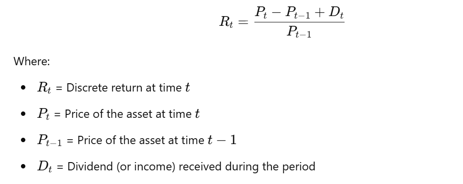
Example:

If an asset's price was $100 yesterday and is $110 today, the discrete return is (110-100)/100 = 0.10 or 10%.

Continuously Compounded Returns

Continuously compounded returns, also known as logarithmic returns, are calculated using the natural logarithm of the price ratio.

Formula:

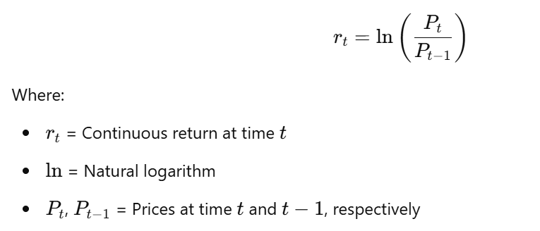
Example:

If an asset's price was $100 yesterday and is $110 today, the continuously compounded return is ln(110/100) = ln(1.1) ≈ 0.0953 or 9.53%.

Why Use Returns Instead of Prices?

• Scale Independence: Returns are scale-independent, making it easier to compare the performance of assets with different price levels. A $1 change in a $10 stock is a very different return than a $1 change in a $1000 stock.
• Aggregation: Returns can be more easily aggregated across time and across assets to calculate portfolio returns.
• Statistical Properties: Returns often exhibit more desirable statistical properties than prices, making them more suitable for econometric modeling. Prices are often non-stationary, while returns can be stationary.

In summary, understanding and calculating both discrete and continuously compounded returns is crucial for anyone working in financial econometrics. The choice between the two often depends on the specific application and the desired properties of the return series.