
Numerical Problem
Identifying and Estimating an ARMA Model
Suppose you have the following sample autocorrelations (ACF) and partial autocorrelations (PACF) for a time series:
| Lag (k) | ACF (ρ_k) | PACF (φ_{kk}) |
|---|---|---|
| 1 | 0.6 | 0.6 |
| 2 | 0.4 | 0.1 |
| 3 | 0.2 | -0.05 |
| 4 | 0.1 | 0.02 |
| 5 | 0.05 | -0.01 |
Based on these ACF and PACF values:
(a) Identify a suitable ARMA model for this time series. (b) Assuming an AR(1) model is appropriate, estimate the AR(1) coefficient.
Solution:
(a) Model Identification:
- ACF Pattern: The ACF decays gradually. This suggests an AR component.
- PACF Pattern: The PACF has a significant spike at lag 1 and then cuts off (or becomes insignificant) after lag 1. This strongly suggests an AR(1) model.
Therefore, a suitable model for this time series is an AR(1) model.
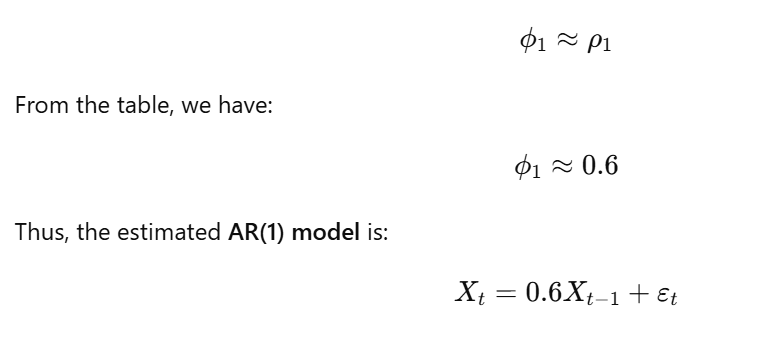
(b) Estimating the AR(1) Coefficient:
For an AR(1) model:

The AR(1) coefficient (φ_1) can be estimated using the sample autocorrelation at lag 1 (ρ_1). In this case, we are given that ρ_1 = 0.6.
Explanation:
-
Why AR(1)? The PACF is key here. The significant spike at lag 1 in the PACF indicates that the correlation between
X_tandX_{t-1}is strong, after removing the effects of intermediate lags. The rapid decay of the PACF after lag 1 suggests that there's no additional direct correlation betweenX_tandX_{t-k}for k > 1, beyond what's already explained byX_{t-1}. -
Estimation: In practice, you would typically estimate the AR(1) coefficient using more sophisticated methods like ordinary least squares (OLS) regression on the time series data. However, in this simplified example, we use the sample autocorrelation as a direct estimate.
Important Considerations (Real World):
-
Statistical Significance: In a real-world scenario, you would need to check the statistical significance of the estimated coefficient. You would calculate a standard error for the estimate and perform a hypothesis test to determine if the coefficient is significantly different from zero.
-
Model Diagnostics: After estimating the model, you would perform diagnostic checks to assess its adequacy. This includes:
- Residual Analysis: Examining the residuals (the difference between the actual values and the values predicted by the model) to see if they resemble white noise. You would check the ACF and PACF of the residuals to look for any remaining autocorrelation.
- Ljung-Box Test: A statistical test for autocorrelation in the residuals.
-
Model Comparison: You might also consider comparing the AR(1) model to other models (e.g., AR(2), ARMA(1,1)) using information criteria like the Akaike Information Criterion (AIC) or the Bayesian Information Criterion (BIC).
This problem illustrates a simplified version of the model identification and estimation steps in the Box-Jenkins approach. The key is to use the ACF and PACF to get an initial idea of the appropriate model order and then to refine the model based on statistical testing and diagnostic checks.
No Comments