Autoregressive (AR), Moving Average (MA), and ARMA Processes

These models are fundamental building blocks in time series analysis. They describe the evolution of a time series based on its past values (AR), past error terms (MA), or a combination of both (ARMA).

1. Autoregressive (AR) Processes

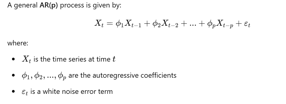
• Definition: An AR process models the current value of a time series as a linear combination of its past values and a white noise error term. The order p of the AR process, denoted as AR(p), indicates the number of past values used in the model.

• Lag Operator Representation:

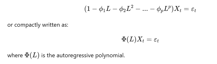
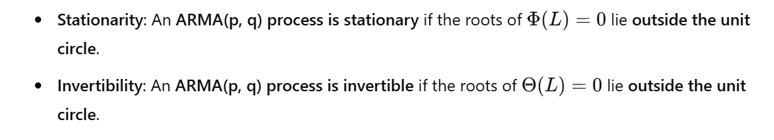
• Stationarity: AR processes are not always stationary. The stationarity of an AR process depends on the roots of the autoregressive polynomial Φ(L). An AR(p) process is stationary if all the roots of Φ(L) = 0 lie outside the unit circle (i.e., have absolute values greater than 1). This is equivalent to saying that all the roots of the characteristic equation Φ(z) = 0 must have absolute values greater than 1, where z = 1/L.

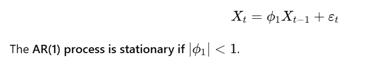
• Example: AR(1) Process:

• ACF and PACF of AR Processes:

  • ACF: The ACF of an AR(p) process decays gradually, often exponentially or in a damped sinusoidal pattern. The decay rate depends on the values of the coefficients φ_1, φ_2, ..., φ_p.
  • PACF: The PACF of an AR(p) process has significant spikes at the first p lags and cuts off to zero after lag p. This property is useful for identifying the order p of an AR process.

2. Moving Average (MA) Processes

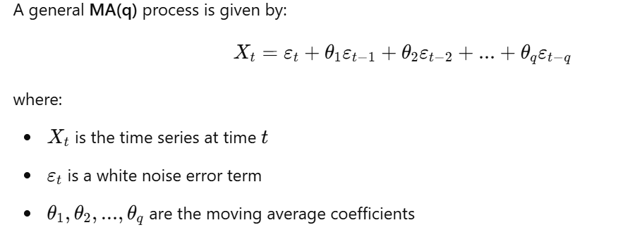
• Definition: An MA process models the current value of a time series as a linear combination of past error terms (white noise). The order q of the MA process, denoted as MA(q), indicates the number of past error terms used in the model.

• MA(q) Model:

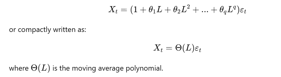
• Lag Operator Representation:

• Stationarity: MA processes are always stationary, regardless of the values of the coefficients θ_1, θ_2, ..., θ_q.

• Invertibility: MA processes may or may not be invertible. An MA(q) process is invertible if all the roots of Θ(L) = 0 lie outside the unit circle. Invertibility is important for forecasting.

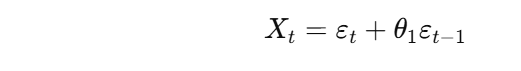
• Example: MA(1) Process:

• ACF and PACF of MA Processes:

  • ACF: The ACF of an MA(q) process has significant spikes at the first q lags and cuts off to zero after lag q. This property is useful for identifying the order q of an MA process.
  • PACF: The PACF of an MA(q) process decays gradually.

3. Autoregressive Moving Average (ARMA) Processes

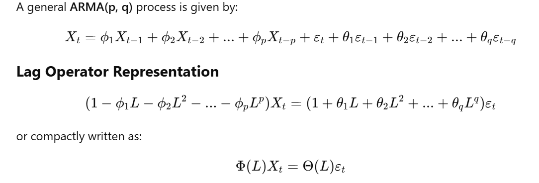
• Definition: An ARMA process combines both AR and MA components. It models the current value of a time series as a linear combination of its past values and past error terms. The order of the ARMA process is denoted as ARMA(p, q), where p is the order of the AR component and q is the order of the MA component.

• ARMA(p, q) Model:

• Stationarity and Invertibility:

• ACF and PACF of ARMA Processes:

  • ACF: The ACF of an ARMA process decays gradually after the first q lags.
  • PACF: The PACF of an ARMA process decays gradually after the first p lags.

  The ACF and PACF patterns of ARMA processes can be more complex than those of pure AR or MA processes, making model identification more challenging.

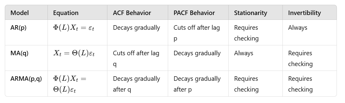
Summary Table: Key Properties

Applications in Finance

AR, MA, and ARMA models can be used to model various financial time series, such as stock returns, interest rates, and exchange rates. However, due to the stylized facts of financial returns (e.g., volatility clustering), more advanced models like GARCH models are often preferred for modeling volatility. ARMA models can still be useful for modeling the mean of a financial time series, while GARCH models capture the variance.