Generalized Autoregressive Conditional Heteroscedasticity (GARCH) Models

GARCH models, introduced by Bollerslev (1986), are an extension of ARCH models that allow the conditional variance to depend on both past squared error terms and past conditional variances. This generalization provides a more flexible and parsimonious way to model volatility clustering and persistence in financial time series. GARCH models are among the most widely used models for volatility forecasting in finance.

Basic Idea

GARCH models build upon the ARCH framework by adding a moving average component to the conditional variance equation. This means that the current conditional variance is a function of both past squared errors (as in ARCH models) and past conditional variances. This allows the model to capture the persistence of volatility more effectively.

GARCH(p, q) Model

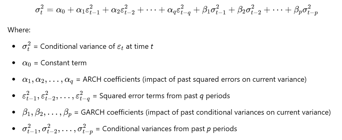
The GARCH(p, q) model specifies that the conditional variance of the error term at time t depends on the q most recent squared error terms and the p most recent conditional variances. The model is defined as follows:

1. Mean Equation:

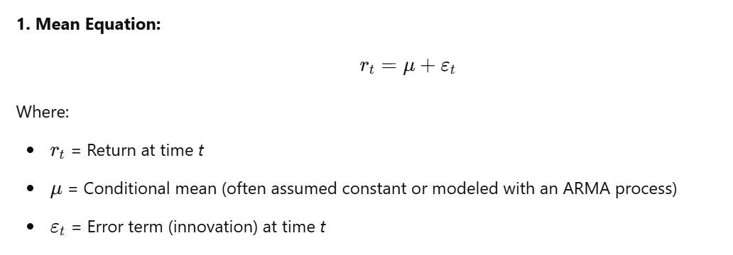
2. Variance Equation (Conditional Variance):

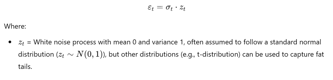
3. Error Term Distribution:

Key Assumptions and Properties

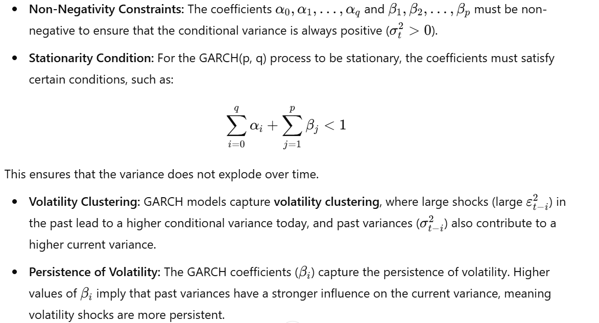
• Symmetric Response: Like ARCH models, GARCH models respond symmetrically to positive and negative shocks. This is a limitation, as it does not capture the leverage effect.

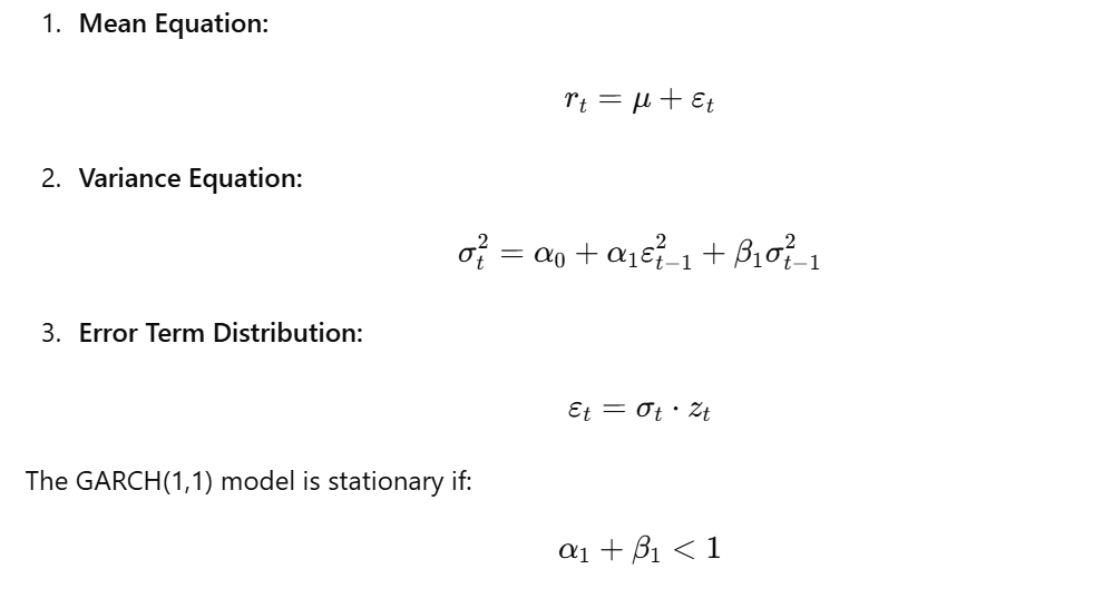
Example: GARCH(1,1) Model

The GARCH(1,1) model is the most widely used GARCH model. It specifies that the conditional variance depends on the most recent squared error term and the most recent conditional variance:

Estimation of GARCH Models

The parameters of GARCH models (μ, α_0, α_1, ..., α_q, β_1, β_2, ..., β_p) are typically estimated using maximum likelihood estimation (MLE). This involves finding the parameter values that maximize the likelihood of observing the given data, given the GARCH model specification.

Model Selection

The orders p and q of the GARCH model can be selected using information criteria, such as the AIC or BIC, or by examining the ACF and PACF of the squared residuals from a simpler model (e.g., an ARMA model for the mean). However, in practice, the GARCH(1,1) model is often chosen due to its simplicity and ability to capture the key features of volatility dynamics.

Advantages of GARCH Models over ARCH Models

• Parsimony: GARCH models can capture the persistence of volatility with fewer parameters than ARCH models. This makes them more efficient and less prone to overfitting.
• Flexibility: GARCH models provide a more flexible framework for modeling volatility dynamics.

Limitations of GARCH Models

• Symmetric Response: Like ARCH models, GARCH models do not capture the asymmetric response of volatility to positive and negative shocks (the leverage effect).
• Parameter Restrictions: The non-negativity constraints on the coefficients can be restrictive.
• Distributional Assumptions: The assumption of a normal distribution for the error term may not be appropriate for all financial time series, especially those with fat tails.

Extensions of GARCH Models

Several extensions of GARCH models have been developed to address these limitations, including:

• EGARCH (Exponential GARCH) Models: Capture the asymmetric response of volatility to positive and negative shocks.
• TARCH (Threshold GARCH) Models: Also capture asymmetric effects.
• FIGARCH (Fractionally Integrated GARCH) Models: Capture long memory in volatility.
• GJR-GARCH Models: Another way to model the asymmetric response of volatility.
• GARCH-M Models: Include the conditional variance (or standard deviation) in the mean equation, allowing volatility to affect the expected return.

Conclusion

GARCH models are a powerful tool for modeling and forecasting volatility in financial time series. They provide a more flexible and parsimonious framework than ARCH models and are widely used in risk management, option pricing, and other financial applications. While they have some limitations, several extensions of GARCH models have been developed to address these limitations and capture more complex volatility dynamics.