Capital Asset Pricing Model (CAPM)

Efficient Frontier with a Combination of Risky and Risk-Free Assets

Core Concept: The Capital Asset Pricing Model (CAPM) is a widely used asset pricing model that describes the relationship between systematic risk and expected return for assets, particularly stocks. It builds upon the concepts of Modern Portfolio Theory (MPT) and introduces the idea of a risk-free asset to determine the efficient frontier and the required rate of return for an investment. 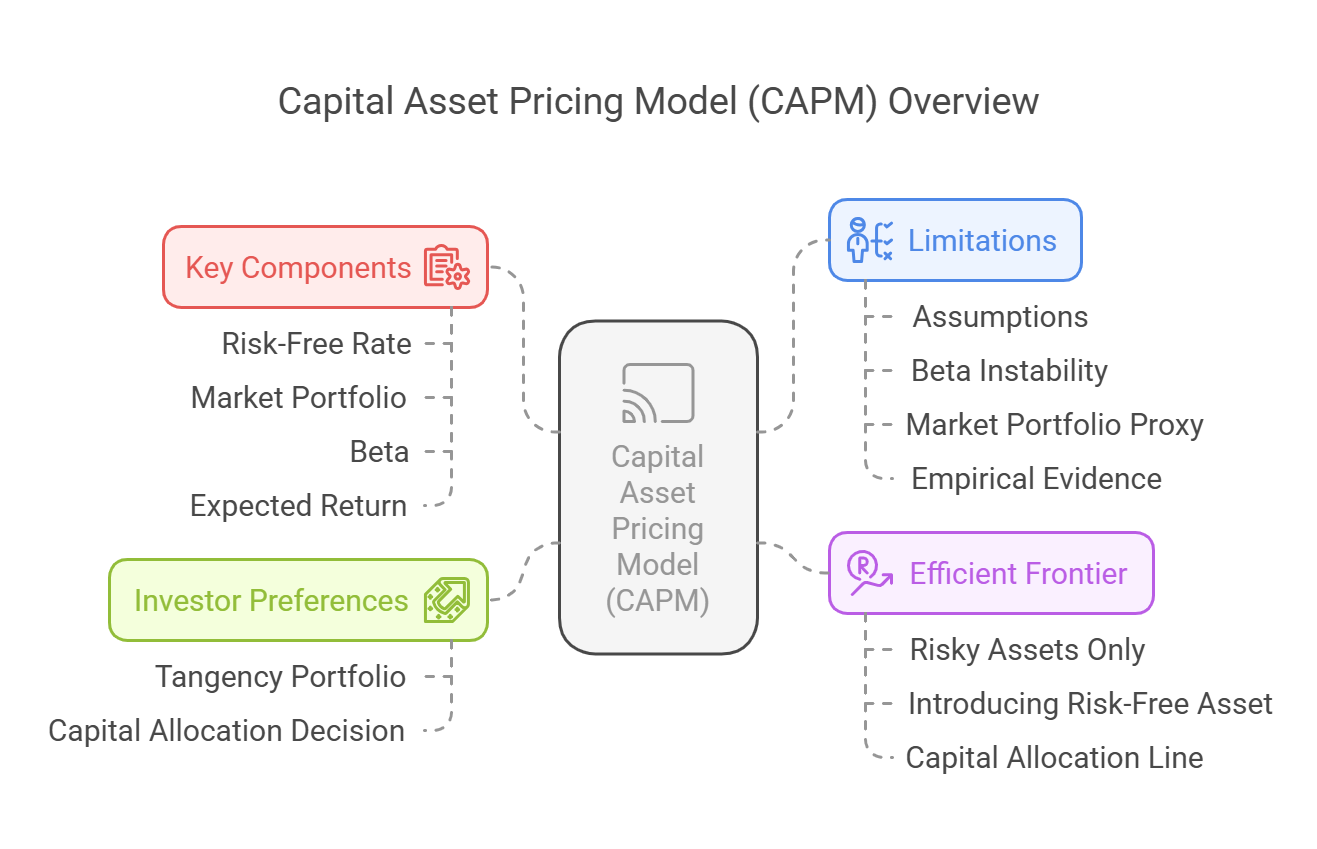Key Components of CAPM:

• Risk-Free Rate (Rf): The rate of return on a risk-free investment, such as a government bond.
• Market Portfolio (M): A portfolio that contains all assets in the market, weighted by their market capitalization. In practice, a broad market index (e.g., S&P 500, NIFTY 50) is often used as a proxy for the market portfolio.
• Beta (β): A measure of an asset's systematic risk or sensitivity to market movements.
• Expected Return (E(Ri)): The anticipated return on an asset.

CAPM Formula:

E(Ri) = Rf + βi * (E(Rm) - Rf)

• Where:
  • E(Ri) = Expected return of asset i
  • Rf = Risk-free rate
  • βi = Beta of asset i
  • E(Rm) = Expected return of the market portfolio
  • (E(Rm) - Rf) = Market risk premium (the additional return investors require for investing in the market portfolio rather than the risk-free asset)

1. Efficient Frontier with Risky Assets Only (Before CAPM)

• In the absence of a risk-free asset, the efficient frontier represents the set of portfolios that offer the highest expected return for a given level of risk, considering only risky assets.
• Investors choose a portfolio on this frontier based on their individual risk preferences.
• The portfolio selection process involves finding the optimal combination of risky assets that maximizes the Sharpe ratio (risk-adjusted return).

2. Introducing the Risk-Free Asset

• The CAPM introduces the concept of a risk-free asset, which is an investment that has a guaranteed return and zero risk of default (e.g., a government treasury bill).
• The risk-free asset can be combined with a portfolio of risky assets to create a new set of investment opportunities.
• By combining the risk-free asset with a risky portfolio, investors can create portfolios with a desired level of risk and return that is different from what is available from the risky assets alone.
• The combination is achieved through leveraging and de-leveraging, described below.

3. Capital Allocation Line (CAL)

• Definition: The Capital Allocation Line (CAL) represents the set of possible combinations of a risk-free asset and a risky portfolio. It is a straight line that connects the risk-free rate (Rf) on the y-axis with the risky portfolio on the efficient frontier.
• Formula: The CAL depicts the risk-return tradeoff that can be achieved by combining the risk-free asset and a risky portfolio.
• Slope of the CAL: The slope of the CAL is the Sharpe ratio of the risky portfolio. It measures the risk-adjusted return of the risky portfolio.
  • Sharpe Ratio = (E(Rp) - Rf) / σp
    • Where:
      • E(Rp) = Expected return of the risky portfolio
      • Rf = Risk-free rate
      • σp = Standard deviation of the risky portfolio
• Leveraging and Deleveraging:
  • Deleveraging (Investing in the Risk-Free Asset): An investor can reduce the risk of their portfolio by allocating a portion of their wealth to the risk-free asset. This is known as deleveraging. It results in a lower expected return but also lower risk. On the CAL graph, this is a point between the Risk Free Rate, and the portfolio (moving towards the risk free rate).
  • Leveraging (Borrowing at the Risk-Free Rate): An investor can increase the potential return of their portfolio by borrowing funds at the risk-free rate and investing those funds in the risky portfolio. This is known as leveraging. It results in a higher expected return but also higher risk. On the CAL graph, this is a point beyond the portfolio (moving away from the risk free rate).
• The Tangency Portfolio:
  • The CAL that offers the highest Sharpe ratio (i.e., the steepest slope) is tangent to the efficient frontier of risky assets. This point of tangency represents the tangency portfolio (T), also known as the market portfolio in CAPM.
  • The tangency portfolio is the most efficient portfolio of risky assets and is the same for all investors, regardless of their risk preferences.

4. The New Efficient Frontier (with a Risk-Free Asset)

• When a risk-free asset is introduced, the efficient frontier changes from a curve (representing combinations of risky assets only) to a straight line (the CAL) that is tangent to the original efficient frontier at the tangency portfolio.
• This new efficient frontier (the CAL) offers a superior risk-return trade-off compared to the original efficient frontier.
• All rational investors will choose to invest in the tangency portfolio and then adjust their overall risk level by allocating a portion of their wealth to the risk-free asset or by leveraging their investment in the tangency portfolio.

5. Investor Preferences and Portfolio Selection under CAPM

• Under the CAPM, the portfolio selection process is separated into two independent steps:
  • Step 1: Identification of the Tangency Portfolio: All investors should invest in the tangency portfolio, regardless of their risk preferences. This portfolio offers the highest Sharpe ratio and the best possible risk-return trade-off for risky assets.
  • Step 2: Capital Allocation Decision: Investors then decide how much to allocate to the tangency portfolio and how much to allocate to the risk-free asset, based on their individual risk tolerance and investment goals.
• Risk-averse investors will allocate a larger portion of their wealth to the risk-free asset, while risk-tolerant investors will allocate a larger portion to the tangency portfolio or even leverage their investment in the tangency portfolio.
• The optimal portfolio for each investor will lie along the CAL, with the specific point determined by their indifference curves (as discussed previously).

Limitations of CAPM:

• Assumptions: The CAPM relies on several assumptions that may not hold true in the real world, including:
  • Investors are rational and risk-averse.
  • Investors have homogenous expectations.
  • There are no transaction costs or taxes.
  • All assets are publicly traded and perfectly divisible.
  • Investors can borrow and lend at the risk-free rate.
• Beta Instability: Beta is not always a stable measure of risk and can change over time.
• Market Portfolio Proxy: The market portfolio is difficult to define and measure in practice, and the use of a proxy index may not accurately reflect the true market portfolio.
• Empirical Evidence: Empirical studies have shown that the CAPM does not always accurately predict asset returns.

Conclusion:

The Capital Asset Pricing Model (CAPM) provides a valuable framework for understanding the relationship between risk and return and for constructing efficient portfolios. By introducing the concept of a risk-free asset and the Capital Allocation Line, the CAPM helps investors to make more informed decisions about asset allocation and portfolio construction. However, it's important to be aware of the limitations of the CAPM and to use it in conjunction with other investment tools and strategies.