Share Valuation

Dividend Discount Models (DDM)

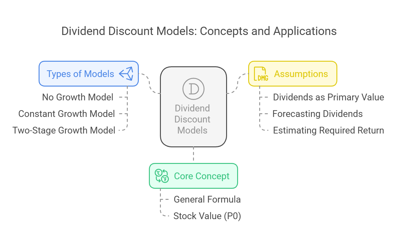
Core Concept: Dividend Discount Models (DDM) are a family of valuation models that determine the intrinsic value of a stock based on the present value of its expected future dividends. The underlying principle is that the value of a stock is the sum of all future dividend payments discounted back to their present value.

General Formula:

Stock Value (P0) = Σ [Dt / (1 + r)^t]

• Where:
  • P0 = Current stock price (intrinsic value)
  • Dt = Expected dividend in year t
  • r = Required rate of return (discount rate)
  • t = Time period (year)
  • Σ = Summation of all future dividends

Assumptions: DDMs rely on certain assumptions, including:

• Dividends are the primary source of value for shareholders.
• Dividends can be reasonably forecasted.
• The required rate of return can be estimated.

Types of Dividend Discount Models:

1. No Growth Model (Zero Growth Model)

• Description: This model assumes that the company will pay a constant dividend forever, with no growth in dividend payments. It is suitable for valuing preferred stocks or mature companies with stable dividend policies and little to no growth prospects.

• Formula:

  P0 = D / r

  • Where:
    • P0 = Current stock price (intrinsic value)
    • D = Constant dividend per share
    • r = Required rate of return

• Example:

  • A company pays a constant dividend of ₹5 per share.
  • The required rate of return is 10%.
  • P0 = ₹5 / 0.10 = ₹50
  • Interpretation: The intrinsic value of the stock is ₹50. An investor should be willing to pay ₹50 for the share.

• Limitations: This model is overly simplistic and rarely applicable to common stocks, as most companies are expected to exhibit some dividend growth over time.

2. Constant Growth Model (Gordon Growth Model)

• Description: This model assumes that dividends will grow at a constant rate forever. It is suitable for valuing companies with a stable history of dividend growth and predictable future growth prospects.

• Formula:

  P0 = D1 / (r - g)

  • Where:
    • P0 = Current stock price (intrinsic value)
    • D1 = Expected dividend per share in the next period (Year 1)
    • r = Required rate of return
    • g = Constant dividend growth rate

• Important Conditions:

  • r > g: The required rate of return must be greater than the dividend growth rate; otherwise, the model produces an unrealistic value.
  • Constant Growth: The growth rate must be sustainable and expected to continue indefinitely.

• Example:

  • A company is expected to pay a dividend of ₹2 per share next year (D1).
  • The required rate of return is 12%.
  • The dividend growth rate is 5%.
  • P0 = ₹2 / (0.12 - 0.05) = ₹2 / 0.07 = ₹28.57
  • Interpretation: The intrinsic value of the stock is approximately ₹28.57.

• Limitations:

  • The assumption of constant growth is often unrealistic, especially for high-growth companies.
  • The model is highly sensitive to changes in the growth rate and required rate of return. Small changes in these inputs can have a significant impact on the estimated stock value.

3. Two-Stage Growth Model

• Description: This model assumes that the company will experience a high growth rate for a specific period, followed by a lower, more sustainable growth rate in the long term. It is suitable for valuing companies that are expected to have a period of rapid growth before transitioning to a more mature stage.

• Formula:

  P0 = Σ [Dt / (1 + r)^t] + [Pn / (1 + r)^n]

  • The formula can be broken down into two stages:
    • Stage 1 (High Growth): Calculate the present value of dividends during the high-growth period (Years 1 to n).
      • Dt = D0 * (1 + gh)^t where D0 is the current dividend and gh is the high growth rate.
    • Stage 2 (Constant Growth): Calculate the present value of the stock price at the end of the high-growth period (Pn), which is calculated using the constant growth model.
      • Pn = Dn+1 / (r - gl) where Dn+1 is the dividend expected in year n+1 and gl is the long-term growth rate.
  • Therefore,

  P0 = Σ [D0 * (1 + gh)^t / (1 + r)^t] + [D0 * (1 + gh)^n * (1 + gl) / (r - gl) / (1 + r)^n]

  • Where:
    • P0 = Current stock price (intrinsic value)
    • D0 = Current dividend per share
    • gh = High dividend growth rate (for the first n years)
    • gl = Long-term dividend growth rate (after year n)
    • r = Required rate of return
    • n = Number of years in the high-growth period

• Example:

  • A company currently pays a dividend of ₹1 per share (D0).
  • The high-growth rate (gh) is 20% for the next 5 years (n = 5).
  • The long-term growth rate (gl) is 5%.
  • The required rate of return (r) is 15%.
  • Calculations:
    • Calculate dividends for years 1 to 5 using D0 * (1 + gh)^t
    • Calculate the terminal stock price (P5) at the end of year 5 using the constant growth model: P5 = D6 / (r - gl)
    • Discount all dividends and the terminal stock price back to the present value.
  • Interpretation: The sum of these present values provides the intrinsic value of the stock.

• Limitations:

  • More complex than the no-growth and constant-growth models, requiring more assumptions.
  • Still sensitive to the accuracy of the growth rate and required rate of return estimates.
  • The choice of the high-growth period (n) can significantly impact the result. Conclusion:

Dividend Discount Models provide a framework for valuing stocks based on the present value of expected future dividends. While each model has its limitations, they can be valuable tools for investors seeking to identify undervalued or overvalued stocks. The choice of which model to use depends on the company's characteristics, dividend policy, and expected growth prospects.